12.2.1 Exercises

1. Using prose, describe how the variables and observations are organised in each of the sample tables.

# table1
# > # A tibble: 6 x 4
# >       country  year  cases population
# >         <chr> <int>  <int>      <int>
# > 1 Afghanistan  1999    745   19987071
# > 2 Afghanistan  2000   2666   20595360
# > 3      Brazil  1999  37737  172006362
# > 4      Brazil  2000  80488  174504898
# > 5       China  1999 212258 1272915272
# > 6       China  2000 213766 1280428583

• table1 is in tidy format. The 4 variables are the columns and each observation is a row.

# table2
#> # A tibble: 12 x 4
#>       country  year       type     count
#>         <chr> <int>      <chr>     <int>
#> 1 Afghanistan  1999      cases       745
#> 2 Afghanistan  1999 population  19987071
#> 3 Afghanistan  2000      cases      2666
#> 4 Afghanistan  2000 population  20595360
#> 5      Brazil  1999      cases     37737
#> 6      Brazil  1999 population 172006362
#> # ... with 6 more rows

• table2 has two variables combined into a single variable type. This means there are twice as many observations as with the tidy data.

# table3
#> # A tibble: 6 x 3
#>       country  year              rate
#> *       <chr> <int>             <chr>
#> 1 Afghanistan  1999      745/19987071
#> 2 Afghanistan  2000     2666/20595360
#> 3      Brazil  1999   37737/172006362
#> 4      Brazil  2000   80488/174504898
#> 5       China  1999 212258/1272915272
#> 6       China  2000 213766/1280428583

• table3 combines the count variable into rate and stores it as a character to maintain to two values for cases and population in the single variable. The labels for those values are no longer in the data.

# Spread across two tibbles
# table4a  # cases
#> # A tibble: 3 x 3
#>       country `1999` `2000`
#> *       <chr>  <int>  <int>
#> 1 Afghanistan    745   2666
#> 2      Brazil  37737  80488
#> 3       China 212258 213766
# table4b  # population
#> # A tibble: 3 x 3
#>       country     `1999`     `2000`
#> *       <chr>      <int>      <int>
#> 1 Afghanistan   19987071   20595360
#> 2      Brazil  172006362  174504898
#> 3       China 1272915272 1280428583

• table4 splits the data into two different tables, a and b. In these tables the years are split into two different variables. There is an observation for each country in these tables.

2. Compute the rate for table2, and table4a + table4b. You will need to perform four operations:

   1. Extract the number of TB cases per country per year.
   2. Extract the matching population per country per year.
   3. Divide cases by population, and multiply by 10000.
   4. Store back in the appropriate place.
      Which representation is easiest to work with? Which is hardest? Why?

table2 <- data_frame(country = c(rep("Afghanistan", 4), rep("Brazil", 4), rep("China", 4)),
                     year = rep(c(1999, 1999, 2000, 2000), 3),
                     type = rep(c("cases", "population"), 6),
                     count = c(745, 19987071, 2666, 20595360, 37737, 172006362, 80488, 174504898, 212258, 1272915272, 213766, 1280428583))

## Warning: `data_frame()` is deprecated, use `tibble()`.
## This warning is displayed once per session.

table2

## # A tibble: 12 x 4
##    country      year type            count
##    <chr>       <dbl> <chr>           <dbl>
##  1 Afghanistan  1999 cases             745
##  2 Afghanistan  1999 population   19987071
##  3 Afghanistan  2000 cases            2666
##  4 Afghanistan  2000 population   20595360
##  5 Brazil       1999 cases           37737
##  6 Brazil       1999 population  172006362
##  7 Brazil       2000 cases           80488
##  8 Brazil       2000 population  174504898
##  9 China        1999 cases          212258
## 10 China        1999 population 1272915272
## 11 China        2000 cases          213766
## 12 China        2000 population 1280428583

(tb_cases <- table2 %>% 
        filter(type %in% "cases"))

## # A tibble: 6 x 4
##   country      year type   count
##   <chr>       <dbl> <chr>  <dbl>
## 1 Afghanistan  1999 cases    745
## 2 Afghanistan  2000 cases   2666
## 3 Brazil       1999 cases  37737
## 4 Brazil       2000 cases  80488
## 5 China        1999 cases 212258
## 6 China        2000 cases 213766

(tb_pop <-  table2 %>% 
        filter(type %in% "population"))

## # A tibble: 6 x 4
##   country      year type            count
##   <chr>       <dbl> <chr>           <dbl>
## 1 Afghanistan  1999 population   19987071
## 2 Afghanistan  2000 population   20595360
## 3 Brazil       1999 population  172006362
## 4 Brazil       2000 population  174504898
## 5 China        1999 population 1272915272
## 6 China        2000 population 1280428583

rate <- tb_cases
rate$rate <- tb_cases$count / tb_pop$count * 10000
rate

## # A tibble: 6 x 5
##   country      year type   count  rate
##   <chr>       <dbl> <chr>  <dbl> <dbl>
## 1 Afghanistan  1999 cases    745 0.373
## 2 Afghanistan  2000 cases   2666 1.29 
## 3 Brazil       1999 cases  37737 2.19 
## 4 Brazil       2000 cases  80488 4.61 
## 5 China        1999 cases 212258 1.67 
## 6 China        2000 cases 213766 1.67

3. Recreate the plot showing change in cases over time using table2 instead of table1. What do you need to do first?

table2 %>% 
        filter(type %in% "cases") %>% 
        ggplot(aes(x = year, y = count)) +
        geom_point(aes(color = country), size = 3) +
        geom_line(aes(group = country))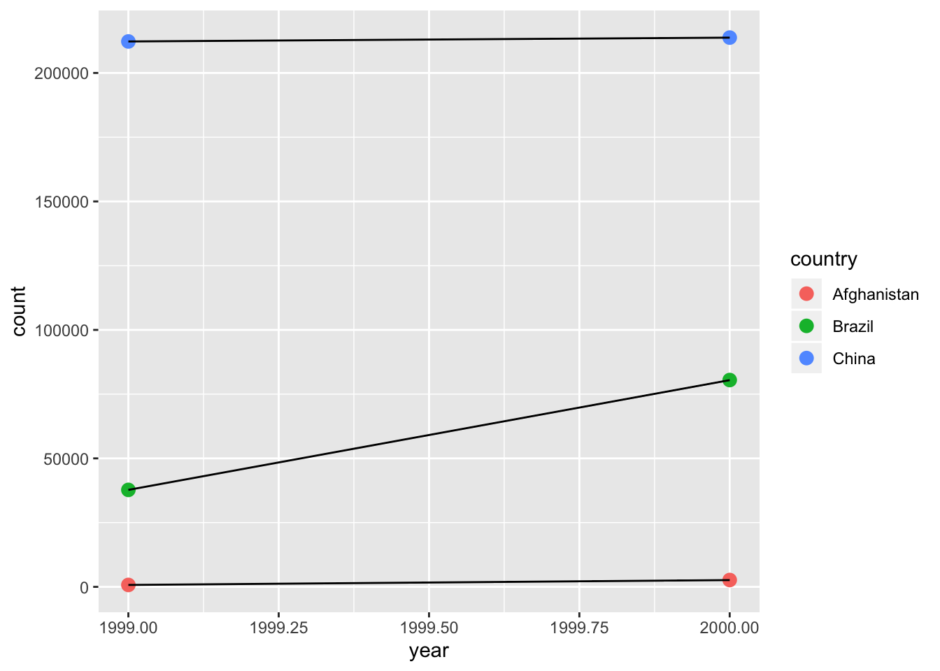

• First you need to filter type for cases.

12.3.3 Exercises

1. Why are gather() and spread() not perfectly symmetrical? Carefully consider the following example:

(stocks <- tibble(
  year   = c(2015, 2015, 2016, 2016),
  half  = c(   1,    2,     1,    2),
  return = c(1.88, 0.59, 0.92, 0.17)
))

## # A tibble: 4 x 3
##    year  half return
##   <dbl> <dbl>  <dbl>
## 1  2015     1   1.88
## 2  2015     2   0.59
## 3  2016     1   0.92
## 4  2016     2   0.17

stocks %>% 
   spread(year, return) %>% 
   gather("year", "return", `2015`:`2016`)

## # A tibble: 4 x 3
##    half year  return
##   <dbl> <chr>  <dbl>
## 1     1 2015    1.88
## 2     2 2015    0.59
## 3     1 2016    0.92
## 4     2 2016    0.17

(Hint: look at the variable types and think about column names.)

Both spread() and gather() have a convert argument. What does it do?

• In the example year is converted to character when it is gathered back after being spread. This happens because convert is by default FALSE so it does not attempt to determine the appropriate class for new columns. When convert is set to TRUE, the year is correctly converted to a number when gathered as seen in the example below.

stocks %>% 
   spread(year, return) %>% 
   gather("year", "return", `2015`:`2016`, convert = TRUE)

## # A tibble: 4 x 3
##    half  year return
##   <dbl> <int>  <dbl>
## 1     1  2015   1.88
## 2     2  2015   0.59
## 3     1  2016   0.92
## 4     2  2016   0.17

2. Why does this code fail?

(table4a <- table2 %>% 
        filter(type %in% "cases") %>% 
        spread(year, count) %>% 
        select(-type))

## # A tibble: 3 x 3
##   country     `1999` `2000`
##   <chr>        <dbl>  <dbl>
## 1 Afghanistan    745   2666
## 2 Brazil       37737  80488
## 3 China       212258 213766

table4a %>%
  gather(1999, 2000, key = "year", value = "cases")

## Error: Can't subset columns that don't exist.
## x The locations 1999 and 2000 don't exist.
## ℹ There are only 3 columns.

• Since the years are numbers they need to be selected with backticks as in the example below.

table4a %>%
  gather(`1999`, `2000`, key = "year", value = "cases", convert = TRUE)

## # A tibble: 6 x 3
##   country      year  cases
##   <chr>       <int>  <dbl>
## 1 Afghanistan  1999    745
## 2 Brazil       1999  37737
## 3 China        1999 212258
## 4 Afghanistan  2000   2666
## 5 Brazil       2000  80488
## 6 China        2000 213766

3. Why does spreading this tibble fail? How could you add a new column to fix the problem?

(people <- tribble(
  ~name,             ~key,    ~value,
  #-----------------|--------|------
  "Phillip Woods",   "age",       45,
  "Phillip Woods",   "height",   186,
  "Phillip Woods",   "age",       50,
  "Jessica Cordero", "age",       37,
  "Jessica Cordero", "height",   156
))

## # A tibble: 5 x 3
##   name            key    value
##   <chr>           <chr>  <dbl>
## 1 Phillip Woods   age       45
## 2 Phillip Woods   height   186
## 3 Phillip Woods   age       50
## 4 Jessica Cordero age       37
## 5 Jessica Cordero height   156

people %>% 
        spread(key, value)

## Error: Each row of output must be identified by a unique combination of keys.
## Keys are shared for 2 rows:
## * 1, 3

• It fails since there are two values for Phillip in age. Fix by adding an index.

(people <- tribble(
  ~name,             ~key,    ~value,  ~index,
  #-----------------|--------|--------|------
  "Phillip Woods",   "age",       45,    1,
  "Phillip Woods",   "height",   186,    1,
  "Phillip Woods",   "age",       50,    2,
  "Jessica Cordero", "age",       37,    1,
  "Jessica Cordero", "height",   156,    1
))

## # A tibble: 5 x 4
##   name            key    value index
##   <chr>           <chr>  <dbl> <dbl>
## 1 Phillip Woods   age       45     1
## 2 Phillip Woods   height   186     1
## 3 Phillip Woods   age       50     2
## 4 Jessica Cordero age       37     1
## 5 Jessica Cordero height   156     1

people %>% 
        spread(key, value)

## # A tibble: 3 x 4
##   name            index   age height
##   <chr>           <dbl> <dbl>  <dbl>
## 1 Jessica Cordero     1    37    156
## 2 Phillip Woods       1    45    186
## 3 Phillip Woods       2    50     NA

4. Tidy the simple tibble below. Do you need to spread or gather it? What are the variables?

preg <- tribble(
  ~pregnant, ~male, ~female,
  "yes",     NA,    10,
  "no",      20,    12
)

preg %>% 
        gather(male, female, key = "sex", value = "count")

## # A tibble: 4 x 3
##   pregnant sex    count
##   <chr>    <chr>  <dbl>
## 1 yes      male      NA
## 2 no       male      20
## 3 yes      female    10
## 4 no       female    12

12.4.3 Exercises

1. What do the extra and fill arguments do in separate()? Experiment with the various options for the following two toy datasets.

tibble(x = c("a,b,c", "d,e,f,g", "h,i,j")) %>% 
  separate(x, c("one", "two", "three"))

## Warning: Expected 3 pieces. Additional pieces discarded in 1 rows [2].

## # A tibble: 3 x 3
##   one   two   three
##   <chr> <chr> <chr>
## 1 a     b     c    
## 2 d     e     f    
## 3 h     i     j

tibble(x = c("a,b,c", "d,e,f,g", "h,i,j")) %>% 
  separate(x, c("one", "two", "three"), extra = "drop")

## # A tibble: 3 x 3
##   one   two   three
##   <chr> <chr> <chr>
## 1 a     b     c    
## 2 d     e     f    
## 3 h     i     j

tibble(x = c("a,b,c", "d,e,f,g", "h,i,j")) %>% 
  separate(x, c("one", "two", "three"), extra = "merge")

## # A tibble: 3 x 3
##   one   two   three
##   <chr> <chr> <chr>
## 1 a     b     c    
## 2 d     e     f,g  
## 3 h     i     j

tibble(x = c("a,b,c", "d,e", "f,g,i")) %>% 
  separate(x, c("one", "two", "three"))

## Warning: Expected 3 pieces. Missing pieces filled with `NA` in 1 rows [2].

## # A tibble: 3 x 3
##   one   two   three
##   <chr> <chr> <chr>
## 1 a     b     c    
## 2 d     e     <NA> 
## 3 f     g     i

tibble(x = c("a,b,c", "d,e", "f,g,i")) %>% 
  separate(x, c("one", "two", "three"), fill = "right")

## # A tibble: 3 x 3
##   one   two   three
##   <chr> <chr> <chr>
## 1 a     b     c    
## 2 d     e     <NA> 
## 3 f     g     i

tibble(x = c("a,b,c", "d,e", "f,g,i")) %>% 
  separate(x, c("one", "two", "three"), fill = "left")

## # A tibble: 3 x 3
##   one   two   three
##   <chr> <chr> <chr>
## 1 a     b     c    
## 2 <NA>  d     e    
## 3 f     g     i

• They control the behavior for when a vector has too many or too few pieces.

2. Both unite() and separate() have a remove argument. What does it do? Why would you set it to FALSE?

• It removes the original column that was modified. Setting to FALSE would allow you to keep the original variable in the data.

3. Compare and contrast separate() and extract(). Why are there three variations of separation (by position, by separator, and with groups), but only one unite?

• extract() separates on a defined regex. There is only one variation for unite() since the columns are already specified and it only requires a separator to be defined. When separating it is more ambiguous so more options are required to cover possibilities.

12.5.1 Exercises

1. Compare and contrast the fill arguments to spread() and complete().

• spread() will replace NA with whatever is specified in fill

• complete() A named list that for each variable supplies a single value to use instead of NA for missing combinations. Like with spread() if specified will replace both explicit and implicit NA

2. What does the direction argument to fill() do?

• Changes which direction to use for the previous entry, default to down.

12.6.1 Exercises

1. In this case study I set na.rm = TRUE just to make it easier to check that we had the correct values. Is this reasonable? Think about how missing values are represented in this dataset. Are there implicit missing values? What’s the difference between an NA and zero?

• In this data NA is assigned to values when there wasn’t a recording for that case in a particular year. A 0 is assigned if the data was recorded but there were no cases. Since there are no implicit missing values it is okay to drop NA.

who %>% 
        count(country) %>% 
        arrange(n) 

## # A tibble: 219 x 2
##    country                               n
##    <chr>                             <int>
##  1 South Sudan                           3
##  2 Bonaire, Saint Eustatius and Saba     4
##  3 Curacao                               4
##  4 Sint Maarten (Dutch part)             4
##  5 Montenegro                            9
##  6 Serbia                                9
##  7 Timor-Leste                          12
##  8 Serbia & Montenegro                  25
##  9 Netherlands Antilles                 30
## 10 Afghanistan                          34
## # … with 209 more rows

who %>% 
        filter(country %in% c("South Sudan",
                              "Bonaire, Saint Eustatius and Saba"))

## # A tibble: 7 x 60
##   country iso2  iso3   year new_sp_m014 new_sp_m1524 new_sp_m2534 new_sp_m3544
##   <chr>   <chr> <chr> <int>       <int>        <int>        <int>        <int>
## 1 Bonair… BQ    BES    2010           0            0            0            0
## 2 Bonair… BQ    BES    2011           0            0            0            0
## 3 Bonair… BQ    BES    2012           0            0            0            0
## 4 Bonair… BQ    BES    2013          NA           NA           NA           NA
## 5 South … SS    SSD    2011          39          251          599          402
## 6 South … SS    SSD    2012          42          356          753          462
## 7 South … SS    SSD    2013          NA           NA           NA           NA
## # … with 52 more variables: new_sp_m4554 <int>, new_sp_m5564 <int>,
## #   new_sp_m65 <int>, new_sp_f014 <int>, new_sp_f1524 <int>,
## #   new_sp_f2534 <int>, new_sp_f3544 <int>, new_sp_f4554 <int>,
## #   new_sp_f5564 <int>, new_sp_f65 <int>, new_sn_m014 <int>,
## #   new_sn_m1524 <int>, new_sn_m2534 <int>, new_sn_m3544 <int>,
## #   new_sn_m4554 <int>, new_sn_m5564 <int>, new_sn_m65 <int>,
## #   new_sn_f014 <int>, new_sn_f1524 <int>, new_sn_f2534 <int>,
## #   new_sn_f3544 <int>, new_sn_f4554 <int>, new_sn_f5564 <int>,
## #   new_sn_f65 <int>, new_ep_m014 <int>, new_ep_m1524 <int>,
## #   new_ep_m2534 <int>, new_ep_m3544 <int>, new_ep_m4554 <int>,
## #   new_ep_m5564 <int>, new_ep_m65 <int>, new_ep_f014 <int>,
## #   new_ep_f1524 <int>, new_ep_f2534 <int>, new_ep_f3544 <int>,
## #   new_ep_f4554 <int>, new_ep_f5564 <int>, new_ep_f65 <int>,
## #   newrel_m014 <int>, newrel_m1524 <int>, newrel_m2534 <int>,
## #   newrel_m3544 <int>, newrel_m4554 <int>, newrel_m5564 <int>,
## #   newrel_m65 <int>, newrel_f014 <int>, newrel_f1524 <int>,
## #   newrel_f2534 <int>, newrel_f3544 <int>, newrel_f4554 <int>,
## #   newrel_f5564 <int>, newrel_f65 <int>

2. What happens if you neglect the mutate() step? (mutate(key = stringr::str_replace(key, “newrel”, “new_rel”)))

• It doesn’t know to separate the values stored as newrel and ends up giving a too few values warning.

who %>%
  gather(code, value, new_sp_m014:newrel_f65, na.rm = TRUE) %>% 
  separate(code, c("new", "var", "sexage")) %>% 
  select(-new, -iso2, -iso3) %>% 
  separate(sexage, c("sex", "age"), sep = 1)

## Warning: Expected 3 pieces. Missing pieces filled with `NA` in 2580 rows [73467,
## 73468, 73469, 73470, 73471, 73472, 73473, 73474, 73475, 73476, 73477, 73478,
## 73479, 73480, 73481, 73482, 73483, 73484, 73485, 73486, ...].

## # A tibble: 76,046 x 6
##    country      year var   sex   age   value
##    <chr>       <int> <chr> <chr> <chr> <int>
##  1 Afghanistan  1997 sp    m     014       0
##  2 Afghanistan  1998 sp    m     014      30
##  3 Afghanistan  1999 sp    m     014       8
##  4 Afghanistan  2000 sp    m     014      52
##  5 Afghanistan  2001 sp    m     014     129
##  6 Afghanistan  2002 sp    m     014      90
##  7 Afghanistan  2003 sp    m     014     127
##  8 Afghanistan  2004 sp    m     014     139
##  9 Afghanistan  2005 sp    m     014     151
## 10 Afghanistan  2006 sp    m     014     193
## # … with 76,036 more rows

3. I claimed that iso2 and iso3 were redundant with country. Confirm this claim.

• There are no additional rows when adding the iso variables to the grouping.

who %>% 
        count(country)

## # A tibble: 219 x 2
##    country                 n
##    <chr>               <int>
##  1 Afghanistan            34
##  2 Albania                34
##  3 Algeria                34
##  4 American Samoa         34
##  5 Andorra                34
##  6 Angola                 34
##  7 Anguilla               34
##  8 Antigua and Barbuda    34
##  9 Argentina              34
## 10 Armenia                34
## # … with 209 more rows

who %>% 
        count(country, iso2, iso3)

## # A tibble: 219 x 4
##    country             iso2  iso3      n
##    <chr>               <chr> <chr> <int>
##  1 Afghanistan         AF    AFG      34
##  2 Albania             AL    ALB      34
##  3 Algeria             DZ    DZA      34
##  4 American Samoa      AS    ASM      34
##  5 Andorra             AD    AND      34
##  6 Angola              AO    AGO      34
##  7 Anguilla            AI    AIA      34
##  8 Antigua and Barbuda AG    ATG      34
##  9 Argentina           AR    ARG      34
## 10 Armenia             AM    ARM      34
## # … with 209 more rows

4. For each country, year, and sex compute the total number of cases of TB. Make an informative visualisation of the data.

who5 %>% 
        filter(sex %in% "f") %>% 
        ggplot(aes(x = year, y = country)) +
        geom_tile(aes(fill = cases)) 

Not actually an informative visualization yet.