
10 Tibbles - R for Data Science
This post covers the content and exercises for Ch 10: Tibbles from R for Data Science. The chapter teaches how to use the tidyverse version of data frames called tibbles.
10.5 Exercises
library(tidyverse)## ── Attaching packages ───────────────────────────────────────────────────────────── tidyverse 1.3.0 ──## ✓ ggplot2 3.2.1 ✓ purrr 0.3.3
## ✓ tibble 2.1.3 ✓ dplyr 0.8.4
## ✓ tidyr 1.0.2 ✓ stringr 1.4.0
## ✓ readr 1.3.1 ✓ forcats 0.4.0## ── Conflicts ──────────────────────────────────────────────────────────────── tidyverse_conflicts() ──
## x dplyr::filter() masks stats::filter()
## x dplyr::lag() masks stats::lag()- How can you tell if an object is a tibble? (Hint: try printing mtcars, which is a regular data frame).
mtcars## mpg cyl disp hp drat wt qsec vs am gear carb
## Mazda RX4 21.0 6 160.0 110 3.90 2.620 16.46 0 1 4 4
## Mazda RX4 Wag 21.0 6 160.0 110 3.90 2.875 17.02 0 1 4 4
## Datsun 710 22.8 4 108.0 93 3.85 2.320 18.61 1 1 4 1
## Hornet 4 Drive 21.4 6 258.0 110 3.08 3.215 19.44 1 0 3 1
## Hornet Sportabout 18.7 8 360.0 175 3.15 3.440 17.02 0 0 3 2
## Valiant 18.1 6 225.0 105 2.76 3.460 20.22 1 0 3 1
## Duster 360 14.3 8 360.0 245 3.21 3.570 15.84 0 0 3 4
## Merc 240D 24.4 4 146.7 62 3.69 3.190 20.00 1 0 4 2
## Merc 230 22.8 4 140.8 95 3.92 3.150 22.90 1 0 4 2
## Merc 280 19.2 6 167.6 123 3.92 3.440 18.30 1 0 4 4
## Merc 280C 17.8 6 167.6 123 3.92 3.440 18.90 1 0 4 4
## Merc 450SE 16.4 8 275.8 180 3.07 4.070 17.40 0 0 3 3
## Merc 450SL 17.3 8 275.8 180 3.07 3.730 17.60 0 0 3 3
## Merc 450SLC 15.2 8 275.8 180 3.07 3.780 18.00 0 0 3 3
## Cadillac Fleetwood 10.4 8 472.0 205 2.93 5.250 17.98 0 0 3 4
## Lincoln Continental 10.4 8 460.0 215 3.00 5.424 17.82 0 0 3 4
## Chrysler Imperial 14.7 8 440.0 230 3.23 5.345 17.42 0 0 3 4
## Fiat 128 32.4 4 78.7 66 4.08 2.200 19.47 1 1 4 1
## Honda Civic 30.4 4 75.7 52 4.93 1.615 18.52 1 1 4 2
## Toyota Corolla 33.9 4 71.1 65 4.22 1.835 19.90 1 1 4 1
## Toyota Corona 21.5 4 120.1 97 3.70 2.465 20.01 1 0 3 1
## Dodge Challenger 15.5 8 318.0 150 2.76 3.520 16.87 0 0 3 2
## AMC Javelin 15.2 8 304.0 150 3.15 3.435 17.30 0 0 3 2
## Camaro Z28 13.3 8 350.0 245 3.73 3.840 15.41 0 0 3 4
## Pontiac Firebird 19.2 8 400.0 175 3.08 3.845 17.05 0 0 3 2
## Fiat X1-9 27.3 4 79.0 66 4.08 1.935 18.90 1 1 4 1
## Porsche 914-2 26.0 4 120.3 91 4.43 2.140 16.70 0 1 5 2
## Lotus Europa 30.4 4 95.1 113 3.77 1.513 16.90 1 1 5 2
## Ford Pantera L 15.8 8 351.0 264 4.22 3.170 14.50 0 1 5 4
## Ferrari Dino 19.7 6 145.0 175 3.62 2.770 15.50 0 1 5 6
## Maserati Bora 15.0 8 301.0 335 3.54 3.570 14.60 0 1 5 8
## Volvo 142E 21.4 4 121.0 109 4.11 2.780 18.60 1 1 4 2as_tibble(mtcars)## # A tibble: 32 x 11
## mpg cyl disp hp drat wt qsec vs am gear carb
## <dbl> <dbl> <dbl> <dbl> <dbl> <dbl> <dbl> <dbl> <dbl> <dbl> <dbl>
## 1 21 6 160 110 3.9 2.62 16.5 0 1 4 4
## 2 21 6 160 110 3.9 2.88 17.0 0 1 4 4
## 3 22.8 4 108 93 3.85 2.32 18.6 1 1 4 1
## 4 21.4 6 258 110 3.08 3.22 19.4 1 0 3 1
## 5 18.7 8 360 175 3.15 3.44 17.0 0 0 3 2
## 6 18.1 6 225 105 2.76 3.46 20.2 1 0 3 1
## 7 14.3 8 360 245 3.21 3.57 15.8 0 0 3 4
## 8 24.4 4 147. 62 3.69 3.19 20 1 0 4 2
## 9 22.8 4 141. 95 3.92 3.15 22.9 1 0 4 2
## 10 19.2 6 168. 123 3.92 3.44 18.3 1 0 4 4
## # … with 22 more rows- One indication is that the rownames are removed from tibbles. When printing to the console it is obvious since the variable classes are displayed under the variable names.
- Compare and contrast the following operations on a data.frame and equivalent tibble. What is different? Why might the default data frame behaviours cause you frustration?
df <- data.frame(abc = 1, xyz = "a")
df$x
## [1] a
## Levels: adf[, "xyz"]## [1] a
## Levels: adf[, c("abc", "xyz")]## abc xyz
## 1 1 adf <- tibble(abc = 1, xyz = "a")
df$x## Warning: Unknown or uninitialised column: 'x'.## NULLdf[, "xyz"]## # A tibble: 1 x 1
## xyz
## <chr>
## 1 adf[, c("abc", "xyz")]## # A tibble: 1 x 2
## abc xyz
## <dbl> <chr>
## 1 1 a- data.frame allows for the partial matching from
$xtoxyz - data.frame converts the text to a factor
- data.frame returns a vector when selecting a single column, while tibble maintains the information in a data frame
- If you have the name of a variable stored in an object, e.g. var <- “mpg”, how can you extract the reference variable from a tibble?
var <- "mpg"
mtcars[[var]]
## [1] 21.0 21.0 22.8 21.4 18.7 18.1 14.3 24.4 22.8 19.2 17.8 16.4 17.3 15.2 10.4
## [16] 10.4 14.7 32.4 30.4 33.9 21.5 15.5 15.2 13.3 19.2 27.3 26.0 30.4 15.8 19.7
## [31] 15.0 21.4Practice referring to non-syntactic names in the following data frame by:
Extracting the variable called 1.
Plotting a scatterplot of 1 vs 2.
Creating a new column called 3 which is 2 divided by 1.
Renaming the columns to one, two and three.
annoying <- tibble(
  `1` = 1:10,
  `2` = `1` * 2 + rnorm(length(`1`))
)

# 1
annoying$`1`
## [1] 1 2 3 4 5 6 7 8 9 10# 2
annoying %>%
ggplot(aes(x = `1`, y = `2`)) +
geom_point()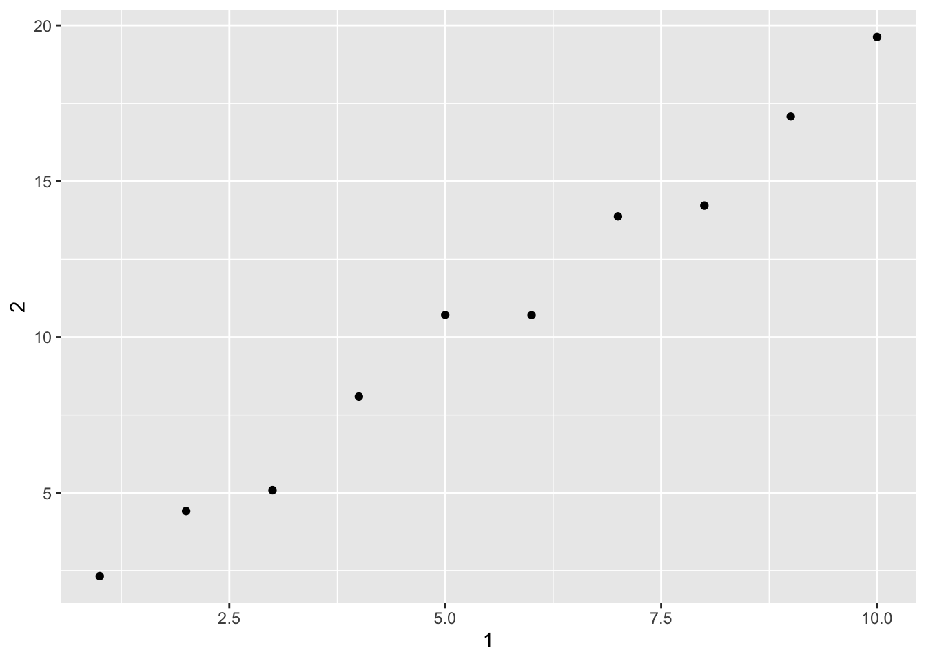
# 3
annoying$`3` <- with(annoying, `2` / `1`)
annoying$`3`
## [1] 2.322234 2.206778 1.693840 2.022740 2.142013 1.784196 1.982088 1.777494
## [9] 1.897767 1.963224# 4
(annoying <- rename(annoying, one = `1`, two = `2`, three = `3`))## # A tibble: 10 x 3
## one two three
## <int> <dbl> <dbl>
## 1 1 2.32 2.32
## 2 2 4.41 2.21
## 3 3 5.08 1.69
## 4 4 8.09 2.02
## 5 5 10.7 2.14
## 6 6 10.7 1.78
## 7 7 13.9 1.98
## 8 8 14.2 1.78
## 9 9 17.1 1.90
## 10 10 19.6 1.96- What does tibble::enframe() do? When might you use it?
enframe(1:3)## # A tibble: 3 x 2
## name value
## <int> <int>
## 1 1 1
## 2 2 2
## 3 3 3c(a = 5, b = 7)## a b
## 5 7enframe(c(a = 5, b = 7))## # A tibble: 2 x 2
## name value
## <chr> <dbl>
## 1 a 5
## 2 b 7- converts named vectors to data frames
- What option controls how many additional column names are printed at the footer of a tibble?
print(as_tibble(mtcars), n_extra = 1)## # A tibble: 32 x 11
## mpg cyl disp hp drat wt qsec vs am gear carb
## <dbl> <dbl> <dbl> <dbl> <dbl> <dbl> <dbl> <dbl> <dbl> <dbl> <dbl>
## 1 21 6 160 110 3.9 2.62 16.5 0 1 4 4
## 2 21 6 160 110 3.9 2.88 17.0 0 1 4 4
## 3 22.8 4 108 93 3.85 2.32 18.6 1 1 4 1
## 4 21.4 6 258 110 3.08 3.22 19.4 1 0 3 1
## 5 18.7 8 360 175 3.15 3.44 17.0 0 0 3 2
## 6 18.1 6 225 105 2.76 3.46 20.2 1 0 3 1
## 7 14.3 8 360 245 3.21 3.57 15.8 0 0 3 4
## 8 24.4 4 147. 62 3.69 3.19 20 1 0 4 2
## 9 22.8 4 141. 95 3.92 3.15 22.9 1 0 4 2
## 10 19.2 6 168. 123 3.92 3.44 18.3 1 0 4 4
## # … with 22 more rows