
5 Data Transformation - R for Data Science
This post covers the content and exercises for Ch 5: Data Transformation from R for Data Science. The chapter teaches how to transform data with dplyr.
5.1 Introduction
5.1.1 Prerequisites
Use data from the nycflights13 package
library(nycflights13)
library(tidyverse)
library(lubridate)
5.1.2 nycflights13
Will be performing data manipulation on nycflights13::flights
flights## # A tibble: 336,776 x 19
## year month day dep_time sched_dep_time dep_delay arr_time sched_arr_time
## <int> <int> <int> <int> <int> <dbl> <int> <int>
## 1 2013 1 1 517 515 2 830 819
## 2 2013 1 1 533 529 4 850 830
## 3 2013 1 1 542 540 2 923 850
## 4 2013 1 1 544 545 -1 1004 1022
## 5 2013 1 1 554 600 -6 812 837
## 6 2013 1 1 554 558 -4 740 728
## 7 2013 1 1 555 600 -5 913 854
## 8 2013 1 1 557 600 -3 709 723
## 9 2013 1 1 557 600 -3 838 846
## 10 2013 1 1 558 600 -2 753 745
## # … with 336,766 more rows, and 11 more variables: arr_delay <dbl>,
## # carrier <chr>, flight <int>, tailnum <chr>, origin <chr>, dest <chr>,
## # air_time <dbl>, distance <dbl>, hour <dbl>, minute <dbl>, time_hour <dttm>5.1.3 dplyr Basics
Will use the 5 common functions of dplyr
filter()for picking observations based on their valuesarrange()for reordering rowsselect()for picking variables by their namemutatefor creating new variables based off of existing variablessummarise()for collapsing many values to a single summary
Can all be used with group_by() which changes scope of each function from entire dataset to going group by group
5.2 Filter Rows with filter()
filter() allows you to subset observations based on their values.
5.2.4 Exercises
- Find all flights that
Had an arrival delay of two or more hours
filter(flights, arr_delay >= 120)## # A tibble: 10,200 x 19
## year month day dep_time sched_dep_time dep_delay arr_time sched_arr_time
## <int> <int> <int> <int> <int> <dbl> <int> <int>
## 1 2013 1 1 811 630 101 1047 830
## 2 2013 1 1 848 1835 853 1001 1950
## 3 2013 1 1 957 733 144 1056 853
## 4 2013 1 1 1114 900 134 1447 1222
## 5 2013 1 1 1505 1310 115 1638 1431
## 6 2013 1 1 1525 1340 105 1831 1626
## 7 2013 1 1 1549 1445 64 1912 1656
## 8 2013 1 1 1558 1359 119 1718 1515
## 9 2013 1 1 1732 1630 62 2028 1825
## 10 2013 1 1 1803 1620 103 2008 1750
## # … with 10,190 more rows, and 11 more variables: arr_delay <dbl>,
## # carrier <chr>, flight <int>, tailnum <chr>, origin <chr>, dest <chr>,
## # air_time <dbl>, distance <dbl>, hour <dbl>, minute <dbl>, time_hour <dttm>Flew to Houston (IAH or HOU)
filter(flights, dest %in% c("IAH", "HOU"))## # A tibble: 9,313 x 19
## year month day dep_time sched_dep_time dep_delay arr_time sched_arr_time
## <int> <int> <int> <int> <int> <dbl> <int> <int>
## 1 2013 1 1 517 515 2 830 819
## 2 2013 1 1 533 529 4 850 830
## 3 2013 1 1 623 627 -4 933 932
## 4 2013 1 1 728 732 -4 1041 1038
## 5 2013 1 1 739 739 0 1104 1038
## 6 2013 1 1 908 908 0 1228 1219
## 7 2013 1 1 1028 1026 2 1350 1339
## 8 2013 1 1 1044 1045 -1 1352 1351
## 9 2013 1 1 1114 900 134 1447 1222
## 10 2013 1 1 1205 1200 5 1503 1505
## # … with 9,303 more rows, and 11 more variables: arr_delay <dbl>,
## # carrier <chr>, flight <int>, tailnum <chr>, origin <chr>, dest <chr>,
## # air_time <dbl>, distance <dbl>, hour <dbl>, minute <dbl>, time_hour <dttm>Were operated by United, American, or Delta
airlines## # A tibble: 16 x 2
## carrier name
## <chr> <chr>
## 1 9E Endeavor Air Inc.
## 2 AA American Airlines Inc.
## 3 AS Alaska Airlines Inc.
## 4 B6 JetBlue Airways
## 5 DL Delta Air Lines Inc.
## 6 EV ExpressJet Airlines Inc.
## 7 F9 Frontier Airlines Inc.
## 8 FL AirTran Airways Corporation
## 9 HA Hawaiian Airlines Inc.
## 10 MQ Envoy Air
## 11 OO SkyWest Airlines Inc.
## 12 UA United Air Lines Inc.
## 13 US US Airways Inc.
## 14 VX Virgin America
## 15 WN Southwest Airlines Co.
## 16 YV Mesa Airlines Inc.filter(flights, carrier %in% c("AA", "DL", "UA"))## # A tibble: 139,504 x 19
## year month day dep_time sched_dep_time dep_delay arr_time sched_arr_time
## <int> <int> <int> <int> <int> <dbl> <int> <int>
## 1 2013 1 1 517 515 2 830 819
## 2 2013 1 1 533 529 4 850 830
## 3 2013 1 1 542 540 2 923 850
## 4 2013 1 1 554 600 -6 812 837
## 5 2013 1 1 554 558 -4 740 728
## 6 2013 1 1 558 600 -2 753 745
## 7 2013 1 1 558 600 -2 924 917
## 8 2013 1 1 558 600 -2 923 937
## 9 2013 1 1 559 600 -1 941 910
## 10 2013 1 1 559 600 -1 854 902
## # … with 139,494 more rows, and 11 more variables: arr_delay <dbl>,
## # carrier <chr>, flight <int>, tailnum <chr>, origin <chr>, dest <chr>,
## # air_time <dbl>, distance <dbl>, hour <dbl>, minute <dbl>, time_hour <dttm>Departed in summer (July, August, and September)
filter(flights, month %in% c(7, 8, 9))## # A tibble: 86,326 x 19
## year month day dep_time sched_dep_time dep_delay arr_time sched_arr_time
## <int> <int> <int> <int> <int> <dbl> <int> <int>
## 1 2013 7 1 1 2029 212 236 2359
## 2 2013 7 1 2 2359 3 344 344
## 3 2013 7 1 29 2245 104 151 1
## 4 2013 7 1 43 2130 193 322 14
## 5 2013 7 1 44 2150 174 300 100
## 6 2013 7 1 46 2051 235 304 2358
## 7 2013 7 1 48 2001 287 308 2305
## 8 2013 7 1 58 2155 183 335 43
## 9 2013 7 1 100 2146 194 327 30
## 10 2013 7 1 100 2245 135 337 135
## # … with 86,316 more rows, and 11 more variables: arr_delay <dbl>,
## # carrier <chr>, flight <int>, tailnum <chr>, origin <chr>, dest <chr>,
## # air_time <dbl>, distance <dbl>, hour <dbl>, minute <dbl>, time_hour <dttm>Arrived more than two hours late, but didn’t leave late
filter(flights, arr_delay >120 & dep_delay <= 0)## # A tibble: 29 x 19
## year month day dep_time sched_dep_time dep_delay arr_time sched_arr_time
## <int> <int> <int> <int> <int> <dbl> <int> <int>
## 1 2013 1 27 1419 1420 -1 1754 1550
## 2 2013 10 7 1350 1350 0 1736 1526
## 3 2013 10 7 1357 1359 -2 1858 1654
## 4 2013 10 16 657 700 -3 1258 1056
## 5 2013 11 1 658 700 -2 1329 1015
## 6 2013 3 18 1844 1847 -3 39 2219
## 7 2013 4 17 1635 1640 -5 2049 1845
## 8 2013 4 18 558 600 -2 1149 850
## 9 2013 4 18 655 700 -5 1213 950
## 10 2013 5 22 1827 1830 -3 2217 2010
## # … with 19 more rows, and 11 more variables: arr_delay <dbl>, carrier <chr>,
## # flight <int>, tailnum <chr>, origin <chr>, dest <chr>, air_time <dbl>,
## # distance <dbl>, hour <dbl>, minute <dbl>, time_hour <dttm>Were delayed by at least an hour, but made up over 30 minutes in flight
filter(flights, dep_delay >= 60 & arr_delay < 30)## # A tibble: 206 x 19
## year month day dep_time sched_dep_time dep_delay arr_time sched_arr_time
## <int> <int> <int> <int> <int> <dbl> <int> <int>
## 1 2013 1 3 1850 1745 65 2148 2120
## 2 2013 1 3 1950 1845 65 2228 2227
## 3 2013 1 3 2015 1915 60 2135 2111
## 4 2013 1 6 1019 900 79 1558 1530
## 5 2013 1 7 1543 1430 73 1758 1735
## 6 2013 1 11 1020 920 60 1311 1245
## 7 2013 1 12 1706 1600 66 1949 1927
## 8 2013 1 12 1953 1845 68 2154 2137
## 9 2013 1 19 1456 1355 61 1636 1615
## 10 2013 1 21 1531 1430 61 1843 1815
## # … with 196 more rows, and 11 more variables: arr_delay <dbl>, carrier <chr>,
## # flight <int>, tailnum <chr>, origin <chr>, dest <chr>, air_time <dbl>,
## # distance <dbl>, hour <dbl>, minute <dbl>, time_hour <dttm>Departed between midnight and 6am (inclusive)
filter(flights, dep_time == 2400 | dep_time <= 0600)## # A tibble: 9,373 x 19
## year month day dep_time sched_dep_time dep_delay arr_time sched_arr_time
## <int> <int> <int> <int> <int> <dbl> <int> <int>
## 1 2013 1 1 517 515 2 830 819
## 2 2013 1 1 533 529 4 850 830
## 3 2013 1 1 542 540 2 923 850
## 4 2013 1 1 544 545 -1 1004 1022
## 5 2013 1 1 554 600 -6 812 837
## 6 2013 1 1 554 558 -4 740 728
## 7 2013 1 1 555 600 -5 913 854
## 8 2013 1 1 557 600 -3 709 723
## 9 2013 1 1 557 600 -3 838 846
## 10 2013 1 1 558 600 -2 753 745
## # … with 9,363 more rows, and 11 more variables: arr_delay <dbl>,
## # carrier <chr>, flight <int>, tailnum <chr>, origin <chr>, dest <chr>,
## # air_time <dbl>, distance <dbl>, hour <dbl>, minute <dbl>, time_hour <dttm>- Another useful dplyr filtering helper is between(). What does it do? Can you use it to simplify the code needed to answer the previous challenges?
between() is a shortcut for x >= left & x <= right
flights[between(flights$dep_time, 0, 600), ]## # A tibble: 17,599 x 19
## year month day dep_time sched_dep_time dep_delay arr_time sched_arr_time
## <int> <int> <int> <int> <int> <dbl> <int> <int>
## 1 2013 1 1 517 515 2 830 819
## 2 2013 1 1 533 529 4 850 830
## 3 2013 1 1 542 540 2 923 850
## 4 2013 1 1 544 545 -1 1004 1022
## 5 2013 1 1 554 600 -6 812 837
## 6 2013 1 1 554 558 -4 740 728
## 7 2013 1 1 555 600 -5 913 854
## 8 2013 1 1 557 600 -3 709 723
## 9 2013 1 1 557 600 -3 838 846
## 10 2013 1 1 558 600 -2 753 745
## # … with 17,589 more rows, and 11 more variables: arr_delay <dbl>,
## # carrier <chr>, flight <int>, tailnum <chr>, origin <chr>, dest <chr>,
## # air_time <dbl>, distance <dbl>, hour <dbl>, minute <dbl>, time_hour <dttm>- How many flights have a missing dep_time? What other variables are missing? What might these rows represent?
filter(flights, is.na(dep_time))## # A tibble: 8,255 x 19
## year month day dep_time sched_dep_time dep_delay arr_time sched_arr_time
## <int> <int> <int> <int> <int> <dbl> <int> <int>
## 1 2013 1 1 NA 1630 NA NA 1815
## 2 2013 1 1 NA 1935 NA NA 2240
## 3 2013 1 1 NA 1500 NA NA 1825
## 4 2013 1 1 NA 600 NA NA 901
## 5 2013 1 2 NA 1540 NA NA 1747
## 6 2013 1 2 NA 1620 NA NA 1746
## 7 2013 1 2 NA 1355 NA NA 1459
## 8 2013 1 2 NA 1420 NA NA 1644
## 9 2013 1 2 NA 1321 NA NA 1536
## 10 2013 1 2 NA 1545 NA NA 1910
## # … with 8,245 more rows, and 11 more variables: arr_delay <dbl>,
## # carrier <chr>, flight <int>, tailnum <chr>, origin <chr>, dest <chr>,
## # air_time <dbl>, distance <dbl>, hour <dbl>, minute <dbl>, time_hour <dttm>Also missing dep_delay, arr_time, arr_delay, air_time, they could represent canceled flights
- Why is NA ^ 0 not missing? Why is NA | TRUE not missing? Why is FALSE & NA not missing? Can you figure out the general rule? (NA * 0 is a tricky counterexample!)
NA ^ 0 # any value ^0 is 1## [1] 1NA | TRUE # Logical is true since one side is true## [1] TRUEFALSE & NA # Logical is false since one side is false## [1] FALSENA * 0 # ???## [1] NAGenerally, operations including NA will be NA unless it would return a specific value no matter what the NA was
5.3 Arrange Rows with arrange()
Arranges a data frame by columns specified, additional columns are used for tie breakers. desc() for descending, and NAs are always pushed to the end
5.3.1 Exercises
- How could you use arrange() to sort all missing values to the start? (Hint: use is.na()).
arrange(flights, desc(is.na(dep_time)))## # A tibble: 336,776 x 19
## year month day dep_time sched_dep_time dep_delay arr_time sched_arr_time
## <int> <int> <int> <int> <int> <dbl> <int> <int>
## 1 2013 1 1 NA 1630 NA NA 1815
## 2 2013 1 1 NA 1935 NA NA 2240
## 3 2013 1 1 NA 1500 NA NA 1825
## 4 2013 1 1 NA 600 NA NA 901
## 5 2013 1 2 NA 1540 NA NA 1747
## 6 2013 1 2 NA 1620 NA NA 1746
## 7 2013 1 2 NA 1355 NA NA 1459
## 8 2013 1 2 NA 1420 NA NA 1644
## 9 2013 1 2 NA 1321 NA NA 1536
## 10 2013 1 2 NA 1545 NA NA 1910
## # … with 336,766 more rows, and 11 more variables: arr_delay <dbl>,
## # carrier <chr>, flight <int>, tailnum <chr>, origin <chr>, dest <chr>,
## # air_time <dbl>, distance <dbl>, hour <dbl>, minute <dbl>, time_hour <dttm>- Sort flights to find the most delayed flights. Find the flights that left earliest.
arrange(flights, desc(dep_delay))## # A tibble: 336,776 x 19
## year month day dep_time sched_dep_time dep_delay arr_time sched_arr_time
## <int> <int> <int> <int> <int> <dbl> <int> <int>
## 1 2013 1 9 641 900 1301 1242 1530
## 2 2013 6 15 1432 1935 1137 1607 2120
## 3 2013 1 10 1121 1635 1126 1239 1810
## 4 2013 9 20 1139 1845 1014 1457 2210
## 5 2013 7 22 845 1600 1005 1044 1815
## 6 2013 4 10 1100 1900 960 1342 2211
## 7 2013 3 17 2321 810 911 135 1020
## 8 2013 6 27 959 1900 899 1236 2226
## 9 2013 7 22 2257 759 898 121 1026
## 10 2013 12 5 756 1700 896 1058 2020
## # … with 336,766 more rows, and 11 more variables: arr_delay <dbl>,
## # carrier <chr>, flight <int>, tailnum <chr>, origin <chr>, dest <chr>,
## # air_time <dbl>, distance <dbl>, hour <dbl>, minute <dbl>, time_hour <dttm>arrange(flights, dep_time)## # A tibble: 336,776 x 19
## year month day dep_time sched_dep_time dep_delay arr_time sched_arr_time
## <int> <int> <int> <int> <int> <dbl> <int> <int>
## 1 2013 1 13 1 2249 72 108 2357
## 2 2013 1 31 1 2100 181 124 2225
## 3 2013 11 13 1 2359 2 442 440
## 4 2013 12 16 1 2359 2 447 437
## 5 2013 12 20 1 2359 2 430 440
## 6 2013 12 26 1 2359 2 437 440
## 7 2013 12 30 1 2359 2 441 437
## 8 2013 2 11 1 2100 181 111 2225
## 9 2013 2 24 1 2245 76 121 2354
## 10 2013 3 8 1 2355 6 431 440
## # … with 336,766 more rows, and 11 more variables: arr_delay <dbl>,
## # carrier <chr>, flight <int>, tailnum <chr>, origin <chr>, dest <chr>,
## # air_time <dbl>, distance <dbl>, hour <dbl>, minute <dbl>, time_hour <dttm>- Sort flights to find the fastest flights.
arrange(flights, air_time)## # A tibble: 336,776 x 19
## year month day dep_time sched_dep_time dep_delay arr_time sched_arr_time
## <int> <int> <int> <int> <int> <dbl> <int> <int>
## 1 2013 1 16 1355 1315 40 1442 1411
## 2 2013 4 13 537 527 10 622 628
## 3 2013 12 6 922 851 31 1021 954
## 4 2013 2 3 2153 2129 24 2247 2224
## 5 2013 2 5 1303 1315 -12 1342 1411
## 6 2013 2 12 2123 2130 -7 2211 2225
## 7 2013 3 2 1450 1500 -10 1547 1608
## 8 2013 3 8 2026 1935 51 2131 2056
## 9 2013 3 18 1456 1329 87 1533 1426
## 10 2013 3 19 2226 2145 41 2305 2246
## # … with 336,766 more rows, and 11 more variables: arr_delay <dbl>,
## # carrier <chr>, flight <int>, tailnum <chr>, origin <chr>, dest <chr>,
## # air_time <dbl>, distance <dbl>, hour <dbl>, minute <dbl>, time_hour <dttm>- Which flights travelled the longest? Which travelled the shortest?
arrange(flights, desc(distance))## # A tibble: 336,776 x 19
## year month day dep_time sched_dep_time dep_delay arr_time sched_arr_time
## <int> <int> <int> <int> <int> <dbl> <int> <int>
## 1 2013 1 1 857 900 -3 1516 1530
## 2 2013 1 2 909 900 9 1525 1530
## 3 2013 1 3 914 900 14 1504 1530
## 4 2013 1 4 900 900 0 1516 1530
## 5 2013 1 5 858 900 -2 1519 1530
## 6 2013 1 6 1019 900 79 1558 1530
## 7 2013 1 7 1042 900 102 1620 1530
## 8 2013 1 8 901 900 1 1504 1530
## 9 2013 1 9 641 900 1301 1242 1530
## 10 2013 1 10 859 900 -1 1449 1530
## # … with 336,766 more rows, and 11 more variables: arr_delay <dbl>,
## # carrier <chr>, flight <int>, tailnum <chr>, origin <chr>, dest <chr>,
## # air_time <dbl>, distance <dbl>, hour <dbl>, minute <dbl>, time_hour <dttm>arrange(flights, distance)## # A tibble: 336,776 x 19
## year month day dep_time sched_dep_time dep_delay arr_time sched_arr_time
## <int> <int> <int> <int> <int> <dbl> <int> <int>
## 1 2013 7 27 NA 106 NA NA 245
## 2 2013 1 3 2127 2129 -2 2222 2224
## 3 2013 1 4 1240 1200 40 1333 1306
## 4 2013 1 4 1829 1615 134 1937 1721
## 5 2013 1 4 2128 2129 -1 2218 2224
## 6 2013 1 5 1155 1200 -5 1241 1306
## 7 2013 1 6 2125 2129 -4 2224 2224
## 8 2013 1 7 2124 2129 -5 2212 2224
## 9 2013 1 8 2127 2130 -3 2304 2225
## 10 2013 1 9 2126 2129 -3 2217 2224
## # … with 336,766 more rows, and 11 more variables: arr_delay <dbl>,
## # carrier <chr>, flight <int>, tailnum <chr>, origin <chr>, dest <chr>,
## # air_time <dbl>, distance <dbl>, hour <dbl>, minute <dbl>, time_hour <dttm>5.4 Select Columns with select()
Helper functions:
* starts_with("abc"): matches names that begin with “abc”.
ends_with("xyz"): matches names that end with “xyz”.contains("ijk"): matches names that contain “ijk”.matches("(.)\\1"): selects variables that match a regular expression. This one matches any variables that contain repeated characters. You’ll learn more about regular expressions in strings.num_range("x", 1:3): matches x1, x2 and x3.
5.4.1 Exercises
- Brainstorm as many ways as possible to select dep_time, dep_delay, arr_time, and arr_delay from flights.
select(flights, dep_time, dep_delay, arr_time, arr_delay)## # A tibble: 336,776 x 4
## dep_time dep_delay arr_time arr_delay
## <int> <dbl> <int> <dbl>
## 1 517 2 830 11
## 2 533 4 850 20
## 3 542 2 923 33
## 4 544 -1 1004 -18
## 5 554 -6 812 -25
## 6 554 -4 740 12
## 7 555 -5 913 19
## 8 557 -3 709 -14
## 9 557 -3 838 -8
## 10 558 -2 753 8
## # … with 336,766 more rows- What happens if you include the name of a variable multiple times in a select() call?
select(flights, dep_time, dep_time)## # A tibble: 336,776 x 1
## dep_time
## <int>
## 1 517
## 2 533
## 3 542
## 4 544
## 5 554
## 6 554
## 7 555
## 8 557
## 9 557
## 10 558
## # … with 336,766 more rows- What does the one_of() function do? Why might it be helpful in conjunction with this vector?
vars <- c("year", "month", "day", "dep_delay", "arr_delay")
vars <- c("year", "month", "day", "dep_delay", "arr_delay")
select(flights, one_of(vars))
## # A tibble: 336,776 x 5
## year month day dep_delay arr_delay
## <int> <int> <int> <dbl> <dbl>
## 1 2013 1 1 2 11
## 2 2013 1 1 4 20
## 3 2013 1 1 2 33
## 4 2013 1 1 -1 -18
## 5 2013 1 1 -6 -25
## 6 2013 1 1 -4 12
## 7 2013 1 1 -5 19
## 8 2013 1 1 -3 -14
## 9 2013 1 1 -3 -8
## 10 2013 1 1 -2 8
## # … with 336,766 more rows- Does the result of running the following code surprise you? How do the select helpers deal with case by default? How can you change that default?
- By default the helpers ignore case, this can be changed by setting
ignore.case = FALSE
select(flights, contains("TIME"))
select(flights, contains("TIME"))## # A tibble: 336,776 x 6
## dep_time sched_dep_time arr_time sched_arr_time air_time time_hour
## <int> <int> <int> <int> <dbl> <dttm>
## 1 517 515 830 819 227 2013-01-01 05:00:00
## 2 533 529 850 830 227 2013-01-01 05:00:00
## 3 542 540 923 850 160 2013-01-01 05:00:00
## 4 544 545 1004 1022 183 2013-01-01 05:00:00
## 5 554 600 812 837 116 2013-01-01 06:00:00
## 6 554 558 740 728 150 2013-01-01 05:00:00
## 7 555 600 913 854 158 2013-01-01 06:00:00
## 8 557 600 709 723 53 2013-01-01 06:00:00
## 9 557 600 838 846 140 2013-01-01 06:00:00
## 10 558 600 753 745 138 2013-01-01 06:00:00
## # … with 336,766 more rows5.5 Add new variables with mutate()
It’s often useful to add new columns that are functions of existing columns. That’s the job of mutate().
5.5.2 Exercises
- Currently dep_time and sched_dep_time are convenient to look at, but hard to compute with because they’re not really continuous numbers. Convert them to a more convenient representation of number of minutes since midnight.
flights_midnight <- flights %>%
  mutate(dep_time_hour = dep_time %/% 100,
       dep_time_min = dep_time %% 100) %>%
  mutate(sched_dep_time_hour = sched_dep_time %/% 100,
         sched_dep_time_min = sched_dep_time %% 100) %>%
  mutate(dep_time_min_mid = dep_time_hour * 60 + dep_time_min,
         sched_dep_time_min_mid = sched_dep_time_hour * 60 + sched_dep_time_min) %>%
  select(-c(dep_time_hour:sched_dep_time_min))
summary(flights_midnight$sched_dep_time_min_mid)
## Min. 1st Qu. Median Mean 3rd Qu. Max.
## 66 546 839 817 1049 1439summary(flights_midnight$dep_time_min_mid)## Min. 1st Qu. Median Mean 3rd Qu. Max. NA's
## 1.0 547.0 841.0 822.2 1064.0 1440.0 8255- Compare air_time with arr_time - dep_time. What do you expect to see? What do you see? What do you need to do to fix it?
flights_midnight %>%
  mutate(air_time_calc = arr_time - dep_time) %>%
  select(air_time, air_time_calc)
## # A tibble: 336,776 x 2
## air_time air_time_calc
## <dbl> <int>
## 1 227 313
## 2 227 317
## 3 160 381
## 4 183 460
## 5 116 258
## 6 150 186
## 7 158 358
## 8 53 152
## 9 140 281
## 10 138 195
## # … with 336,766 more rowsThese should be the same, the issue is that arr_time and dep_time are not currently continuous values so they cannot be subtracted. Fix by using time from midnight for both arr and dep
flights_midnight <- flights_midnight %>%
  mutate(arr_time_hour = arr_time %/% 100,
       arr_time_min = arr_time %% 100) %>%
  mutate(sched_arr_time_hour = sched_arr_time %/% 100,
         sched_arr_time_min = sched_arr_time %% 100) %>%
  mutate(arr_time_min_mid = arr_time_hour * 60 + arr_time_min,
         sched_arr_time_min_mid = sched_arr_time_hour * 60 + sched_arr_time_min) %>%
  select(-c(arr_time_hour:sched_arr_time_min))
summary(flights_midnight$arr_time_min_mid)
## Min. 1st Qu. Median Mean 3rd Qu. Max. NA's
## 1 664 935 913 1180 1440 8713summary(flights_midnight$sched_arr_time_min_mid)## Min. 1st Qu. Median Mean 3rd Qu. Max.
## 1.0 684.0 956.0 933.4 1185.0 1439.0flights_midnight %>%
mutate(air_time_calc = arr_time_min_mid - dep_time_min_mid) %>%
select(air_time, air_time_calc, arr_time_min_mid, dep_time_min_mid) %>%
filter(air_time_calc > 0, !is.na(air_time_calc), !is.na(air_time)) %>%
sample_n(10000) %>%
ggplot() + geom_point(aes(x = air_time, y = air_time_calc), alpha = 0.1)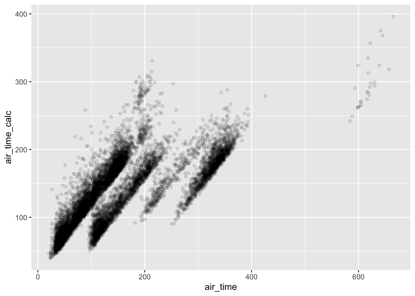
- Can’t explain the offsets
- Compare dep_time, sched_dep_time, and dep_delay. How would you expect those three numbers to be related?
- dep_time should be sched_dep_time + dep_delay after converting to continuous
flights_midnight %>%
  mutate(dep_time_calc = sched_dep_time_min_mid + dep_delay) %>%
  select(dep_time_min_mid, dep_time_calc) %>%
  filter(dep_time_calc < 1440) %>%
  sample_n(5000) %>%
  ggplot() + geom_point(aes(x = dep_time_min_mid, y = dep_time_calc))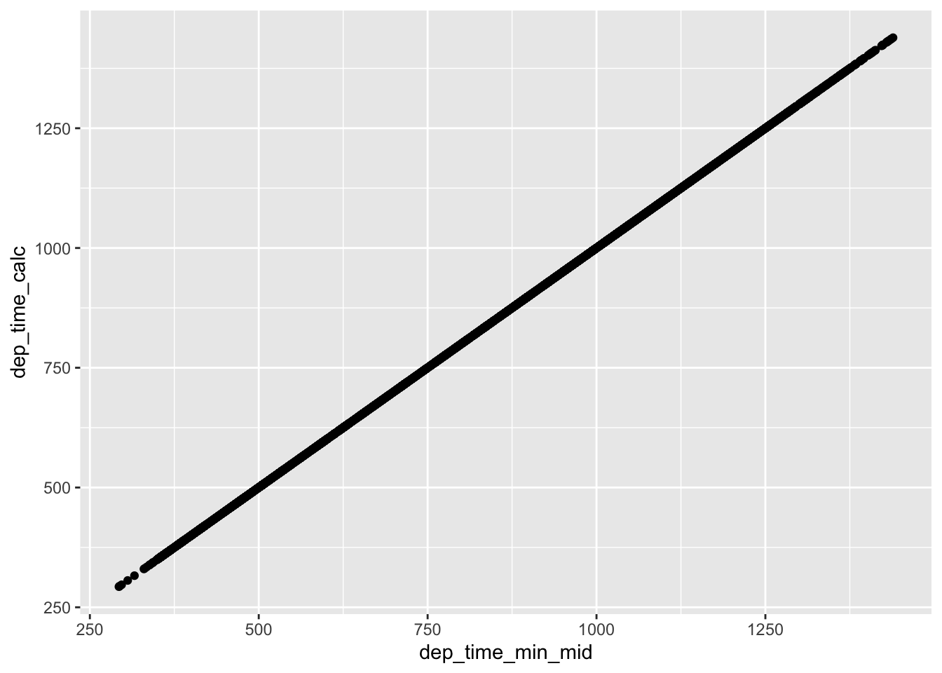
- Find the 10 most delayed flights using a ranking function. How do you want to handle ties? Carefully read the documentation for min_rank().
- I’m using min_rank so ties are returned with the rank equal to the lowest rank value (as in sports)
flights_midnight %>%
  select(dep_delay, tailnum) %>%
  mutate(rank = min_rank(desc(dep_delay))) %>%
  arrange(min_rank(desc(dep_delay))) %>%
  slice(1:10)
## # A tibble: 10 x 3
## dep_delay tailnum rank
## <dbl> <chr> <int>
## 1 1301 N384HA 1
## 2 1137 N504MQ 2
## 3 1126 N517MQ 3
## 4 1014 N338AA 4
## 5 1005 N665MQ 5
## 6 960 N959DL 6
## 7 911 N927DA 7
## 8 899 N3762Y 8
## 9 898 N6716C 9
## 10 896 N5DMAA 10- What does 1:3 + 1:10 return? Why?
1:3 + 1:10## Warning in 1:3 + 1:10: longer object length is not a multiple of shorter object
## length## [1] 2 4 6 5 7 9 8 10 12 11- The first 3 values are added however the remaining values are unchanged and a warning is given since the smaller vector is not a multiple of the longer vector
- What trigonometric functions does R provide?
#?Trig5.6 Grouped Summaries with summarise()
summarise() collapses a data frame into a single row
5.6.7 Exercises
Brainstorm at least 5 different ways to assess the typical delay characteristics of a group of flights. Consider the following scenarios:
- A flight is 15 minutes early 50% of the time, and 15 minutes late 50% of the time.
flights %>%
  group_by(flight) %>%
  summarize(early_15_min = sum(arr_delay <= -15, na.rm = TRUE) / n(),
            late_15_min = sum(arr_delay >= 15, na.rm = TRUE) / n(),
            n = n()) %>%
  filter(early_15_min == 0.5,
         late_15_min == 0.5)
## # A tibble: 18 x 4
## flight early_15_min late_15_min n
## <int> <dbl> <dbl> <int>
## 1 107 0.5 0.5 2
## 2 2072 0.5 0.5 2
## 3 2366 0.5 0.5 2
## 4 2500 0.5 0.5 2
## 5 2552 0.5 0.5 2
## 6 3495 0.5 0.5 2
## 7 3518 0.5 0.5 2
## 8 3544 0.5 0.5 2
## 9 3651 0.5 0.5 2
## 10 3705 0.5 0.5 2
## 11 3916 0.5 0.5 2
## 12 3951 0.5 0.5 2
## 13 4273 0.5 0.5 2
## 14 4313 0.5 0.5 2
## 15 5297 0.5 0.5 2
## 16 5322 0.5 0.5 2
## 17 5388 0.5 0.5 2
## 18 5505 0.5 0.5 4* A flight is always 10 minutes late.flights %>%
group_by(flight) %>%
summarise(prop.same.late = n_distinct(arr_delay, na.rm = TRUE) / n(),
mean.arr.delay = mean(arr_delay, na.rm = TRUE),
n = n()) %>%
filter(prop.same.late == 1 & mean.arr.delay == 10)## # A tibble: 4 x 4
## flight prop.same.late mean.arr.delay n
## <int> <dbl> <dbl> <int>
## 1 2254 1 10 1
## 2 3656 1 10 1
## 3 3880 1 10 1
## 4 5854 1 10 1* A flight is 30 minutes early 50% of the time, and 30 minutes late 50% of the time.flights %>%
group_by(flight) %>%
summarise(early.30.prop = sum(arr_delay <= -30, na.rm = TRUE) / n(),
late.30.prop = sum(arr_delay >= 30, na.rm = TRUE) / n(),
n = n()) %>%
filter(early.30.prop == .5 & late.30.prop == .5)## # A tibble: 3 x 4
## flight early.30.prop late.30.prop n
## <int> <dbl> <dbl> <int>
## 1 3651 0.5 0.5 2
## 2 3916 0.5 0.5 2
## 3 3951 0.5 0.5 2* 99% of the time a flight is on time. 1% of the time it’s 2 hours late.flights %>%
group_by(flight) %>%
summarise(early.prop = sum(arr_delay <= 0, na.rm = TRUE) / n(),
late.prop = sum(arr_delay >= 120, na.rm = TRUE) / n(),
n = n()) %>%
filter(early.prop == .99 & late.prop == .01 )## # A tibble: 0 x 4
## # … with 4 variables: flight <int>, early.prop <dbl>, late.prop <dbl>, n <int>Which is more important: arrival delay or departure delay?
* Arrival delay is more important since it affects making connections and schedules. Departure delay only affect wait time in the ariport
- Come up with another approach that will give you the same output as not_cancelled %>% count(dest) and not_cancelled %>% count(tailnum, wt = distance) (without using count()).
not_cancelled <- flights %>%
        filter(!is.na(dep_time))

not_cancelled %>% count(dest)
## # A tibble: 104 x 2
## dest n
## <chr> <int>
## 1 ABQ 254
## 2 ACK 265
## 3 ALB 419
## 4 ANC 8
## 5 ATL 16898
## 6 AUS 2418
## 7 AVL 263
## 8 BDL 412
## 9 BGR 360
## 10 BHM 272
## # … with 94 more rowsnot_cancelled %>%
group_by(dest) %>%
summarise(n = n())## # A tibble: 104 x 2
## dest n
## <chr> <int>
## 1 ABQ 254
## 2 ACK 265
## 3 ALB 419
## 4 ANC 8
## 5 ATL 16898
## 6 AUS 2418
## 7 AVL 263
## 8 BDL 412
## 9 BGR 360
## 10 BHM 272
## # … with 94 more rowsnot_cancelled %>% count(tailnum, wt = distance)## # A tibble: 4,037 x 2
## tailnum n
## <chr> <dbl>
## 1 D942DN 3418
## 2 N0EGMQ 240626
## 3 N10156 110389
## 4 N102UW 25722
## 5 N103US 24619
## 6 N104UW 25157
## 7 N10575 141475
## 8 N105UW 23618
## 9 N107US 21677
## 10 N108UW 32070
## # … with 4,027 more rowsnot_cancelled %>%
group_by(tailnum) %>%
summarise(n = sum(distance))## # A tibble: 4,037 x 2
## tailnum n
## <chr> <dbl>
## 1 D942DN 3418
## 2 N0EGMQ 240626
## 3 N10156 110389
## 4 N102UW 25722
## 5 N103US 24619
## 6 N104UW 25157
## 7 N10575 141475
## 8 N105UW 23618
## 9 N107US 21677
## 10 N108UW 32070
## # … with 4,027 more rows- Our definition of cancelled flights (is.na(dep_delay) | is.na(arr_delay) ) is slightly suboptimal. Why? Which is the most important column?
flights %>%
  filter(is.na(dep_delay) & !is.na(arr_delay))
## # A tibble: 0 x 19
## # … with 19 variables: year <int>, month <int>, day <int>, dep_time <int>,
## # sched_dep_time <int>, dep_delay <dbl>, arr_time <int>,
## # sched_arr_time <int>, arr_delay <dbl>, carrier <chr>, flight <int>,
## # tailnum <chr>, origin <chr>, dest <chr>, air_time <dbl>, distance <dbl>,
## # hour <dbl>, minute <dbl>, time_hour <dttm>There are no flights which had a NA departure and an arrival time, so we can simplify to only filter for non-NA departures
- Look at the number of cancelled flights per day. Is there a pattern? Is the proportion of cancelled flights related to the average delay?
flights %>%
  mutate(date = ymd(paste(year, month, day))) %>%
  group_by(year, month, day) %>%
  summarise(canceled = sum(is.na(dep_time)),
            date = first(date),
            avg.delay = mean(arr_delay, na.rm = TRUE)) %>%
  ggplot() +
  geom_line(aes(x = date, y = canceled)) +
  geom_line(aes(x = date, y = avg.delay), color = "red")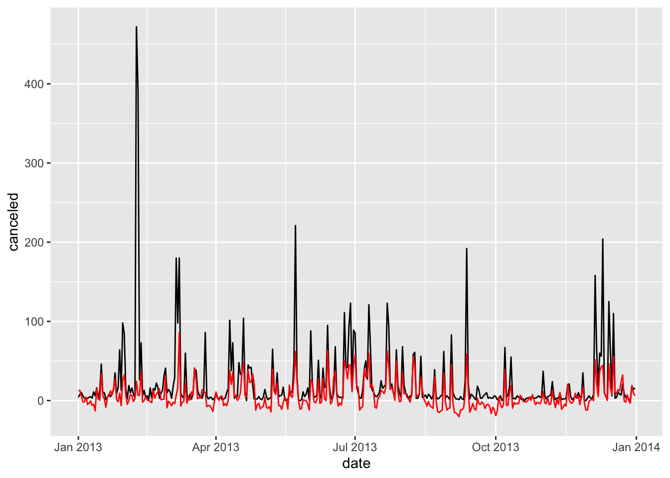
flights %>%
  mutate(date = ymd(paste(year, month, day))) %>%
  group_by(year, month, day) %>%
  summarise(canceled = sum(is.na(dep_time)),
            date = first(date),
            avg.delay = mean(arr_delay, na.rm = TRUE)) %>%
  ggplot(aes(x = log(canceled), y = avg.delay)) +
  geom_point() +
  geom_smooth(method = "lm", se = FALSE)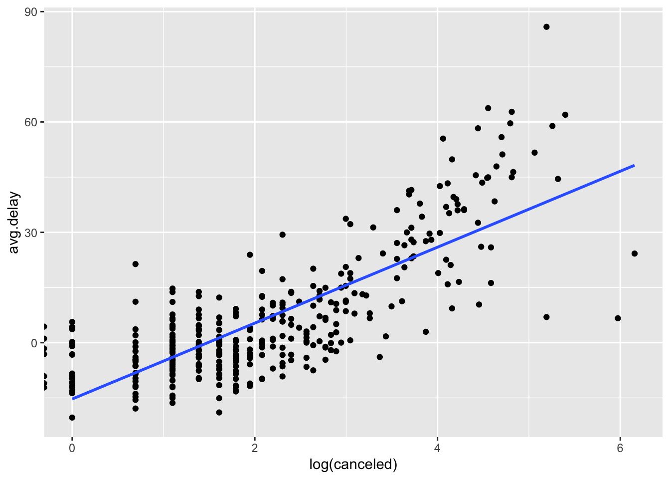
- Yes, there appears to be a relationship between the number of canceled flights and the average delay
- Which carrier has the worst delays? Challenge: can you disentangle the effects of bad airports vs. bad carriers? Why/why not? (Hint: think about flights %>% group_by(carrier, dest) %>% summarise(n()))
flights %>%
  group_by(carrier) %>%
  summarise(avg.delay = mean(arr_delay, na.rm = TRUE)) %>%
  arrange(desc(avg.delay))
## # A tibble: 16 x 2
## carrier avg.delay
## <chr> <dbl>
## 1 F9 21.9
## 2 FL 20.1
## 3 EV 15.8
## 4 YV 15.6
## 5 OO 11.9
## 6 MQ 10.8
## 7 WN 9.65
## 8 B6 9.46
## 9 9E 7.38
## 10 UA 3.56
## 11 US 2.13
## 12 VX 1.76
## 13 DL 1.64
## 14 AA 0.364
## 15 HA -6.92
## 16 AS -9.93flights %>%
group_by(dest) %>%
summarise(avg.delay = mean(arr_delay, na.rm = TRUE),
n = n()) %>%
arrange(desc(avg.delay))## # A tibble: 105 x 3
## dest avg.delay n
## <chr> <dbl> <int>
## 1 CAE 41.8 116
## 2 TUL 33.7 315
## 3 OKC 30.6 346
## 4 JAC 28.1 25
## 5 TYS 24.1 631
## 6 MSN 20.2 572
## 7 RIC 20.1 2454
## 8 CAK 19.7 864
## 9 DSM 19.0 569
## 10 GRR 18.2 765
## # … with 95 more rows- Average delays vary depending on the destination airport. I will attempt to separate airport effects by considering only destinations where each airline made a significant number of stops, and then randomly sample flights to hold the destination constant.
flights %>%
        group_by(dest) %>%
        summarise(num = length(unique(carrier))) %>%
        arrange(desc(num))
## # A tibble: 105 x 2
## dest num
## <chr> <int>
## 1 ATL 7
## 2 BOS 7
## 3 CLT 7
## 4 ORD 7
## 5 TPA 7
## 6 AUS 6
## 7 DCA 6
## 8 DTW 6
## 9 IAD 6
## 10 MSP 6
## # … with 95 more rows- There are no airports that had flights from every carrier. Instead I will use only the destinations that had a low average delay so I can assume differences between destinations will be negligable.
low_delay_dests <- flights %>%
  group_by(dest) %>%
  summarise(avg.delay = mean(arr_delay, na.rm = TRUE),
            n = n()) %>%
filter(avg.delay > -2 & avg.delay < 12)- Confirm all carriers are still in the data set
flights %>%
        filter(dest %in% low_delay_dests$dest) %>%
        count(carrier)
## # A tibble: 16 x 2
## carrier n
## <chr> <int>
## 1 9E 14005
## 2 AA 32426
## 3 AS 714
## 4 B6 53676
## 5 DL 47991
## 6 EV 32243
## 7 F9 685
## 8 FL 2337
## 9 HA 342
## 10 MQ 25861
## 11 OO 31
## 12 UA 57614
## 13 US 20535
## 14 VX 5143
## 15 WN 6852
## 16 YV 290- This leaves 71 destinations with low average delays. Now I can recheck the carriers average delays.
# Results with all destinations
flights %>%
  group_by(carrier) %>%
  summarise(avg.delay = mean(arr_delay, na.rm = TRUE),
            n = n()) %>%
  arrange(desc(avg.delay))
## # A tibble: 16 x 3
## carrier avg.delay n
## <chr> <dbl> <int>
## 1 F9 21.9 685
## 2 FL 20.1 3260
## 3 EV 15.8 54173
## 4 YV 15.6 601
## 5 OO 11.9 32
## 6 MQ 10.8 26397
## 7 WN 9.65 12275
## 8 B6 9.46 54635
## 9 9E 7.38 18460
## 10 UA 3.56 58665
## 11 US 2.13 20536
## 12 VX 1.76 5162
## 13 DL 1.64 48110
## 14 AA 0.364 32729
## 15 HA -6.92 342
## 16 AS -9.93 714# Results filtered for low delay destinations
flights %>%
filter(dest %in% low_delay_dests$dest) %>%
group_by(carrier) %>%
summarise(avg.delay = mean(arr_delay, na.rm = TRUE),
n = n()) %>%
arrange(desc(avg.delay))## # A tibble: 16 x 3
## carrier avg.delay n
## <chr> <dbl> <int>
## 1 F9 21.9 685
## 2 FL 20.7 2337
## 3 EV 13.9 32243
## 4 OO 12.2 31
## 5 YV 12.0 290
## 6 MQ 10.6 25861
## 7 B6 9.40 53676
## 8 WN 8.49 6852
## 9 9E 8.01 14005
## 10 UA 3.73 57614
## 11 US 2.13 20535
## 12 VX 1.82 5143
## 13 DL 1.68 47991
## 14 AA 0.411 32426
## 15 HA -6.92 342
## 16 AS -9.93 714- Filtering out the destinations with high average delays doesn’t have a large effect on the rankings. F9 (Frontier) is still the worst airline with an average delay of 21.9 minutes
- What does the sort argument to count() do. When might you use it?
flights %>%
        count(dest, sort = TRUE)
## # A tibble: 105 x 2
## dest n
## <chr> <int>
## 1 ORD 17283
## 2 ATL 17215
## 3 LAX 16174
## 4 BOS 15508
## 5 MCO 14082
## 6 CLT 14064
## 7 SFO 13331
## 8 FLL 12055
## 9 MIA 11728
## 10 DCA 9705
## # … with 95 more rows- The results are automatically sorted into descending order
5.7 Grouped Mutates (and Filters)
Grouping is most useful in conjunction with summarise(), but you can also do convenient operations with mutate() and filter()
5.7.1 Exercises
Refer back to the lists of useful mutate and filtering functions. Describe how each operation changes when you combine it with grouping.
Which plane (tailnum) has the worst on-time record?
flights %>%
        group_by(tailnum) %>%
        summarise(avg.delay = mean(arr_delay, na.rm = TRUE), n = n()) %>%
        arrange(desc(avg.delay))
## # A tibble: 4,044 x 3
## tailnum avg.delay n
## <chr> <dbl> <int>
## 1 N844MH 320 1
## 2 N911DA 294 1
## 3 N922EV 276 1
## 4 N587NW 264 1
## 5 N851NW 219 1
## 6 N928DN 201 1
## 7 N7715E 188 1
## 8 N654UA 185 1
## 9 N665MQ 175. 6
## 10 N427SW 157 1
## # … with 4,034 more rows- What time of day should you fly if you want to avoid delays as much as possible?
flights_midnight %>%
        group_by(hour) %>%
        summarise(avg.delay = mean(arr_delay, na.rm = TRUE)) %>%
        arrange(avg.delay)
## # A tibble: 20 x 2
## hour avg.delay
## <dbl> <dbl>
## 1 7 -5.30
## 2 5 -4.80
## 3 6 -3.38
## 4 9 -1.45
## 5 8 -1.11
## 6 10 0.954
## 7 11 1.48
## 8 12 3.49
## 9 13 6.54
## 10 14 9.20
## 11 23 11.8
## 12 15 12.3
## 13 16 12.6
## 14 18 14.8
## 15 22 16.0
## 16 17 16.0
## 17 19 16.7
## 18 20 16.7
## 19 21 18.4
## 20 1 NaN- Early morning flights are the best, between 5-7am.
- For each destination, compute the total minutes of delay. For each, flight, compute the proportion of the total delay for its destination.
flights %>%
        group_by(dest) %>%
        filter(arr_delay > 0) %>%
        mutate(tot.delay = sum(arr_delay),
               prop.delay = arr_delay / tot.delay) %>%
        select(year:day, dest, arr_delay, tot.delay, prop.delay)
## # A tibble: 133,004 x 7
## # Groups: dest [103]
## year month day dest arr_delay tot.delay prop.delay
## <int> <int> <int> <chr> <dbl> <dbl> <dbl>
## 1 2013 1 1 IAH 11 99391 0.000111
## 2 2013 1 1 IAH 20 99391 0.000201
## 3 2013 1 1 MIA 33 140424 0.000235
## 4 2013 1 1 ORD 12 283046 0.0000424
## 5 2013 1 1 FLL 19 202605 0.0000938
## 6 2013 1 1 ORD 8 283046 0.0000283
## 7 2013 1 1 LAX 7 203226 0.0000344
## 8 2013 1 1 DFW 31 110009 0.000282
## 9 2013 1 1 ATL 12 300299 0.0000400
## 10 2013 1 1 DTW 16 138258 0.000116
## # … with 132,994 more rows- Delays are typically temporally correlated: even once the problem that caused the initial delay has been resolved, later flights are delayed to allow earlier flights to leave. Using lag() explore how the delay of a flight is related to the delay of the immediately preceding flight.
flights_midnight %>%
        group_by(origin) %>%
        arrange(year, month, day, dep_time_min_mid) %>%
        filter(!is.na(dep_delay)) %>%
        mutate(prev.delay = lag(dep_delay)) %>%
        ggplot(aes(x = dep_delay, y = prev.delay)) +
        geom_point() +
        geom_smooth(method = "lm")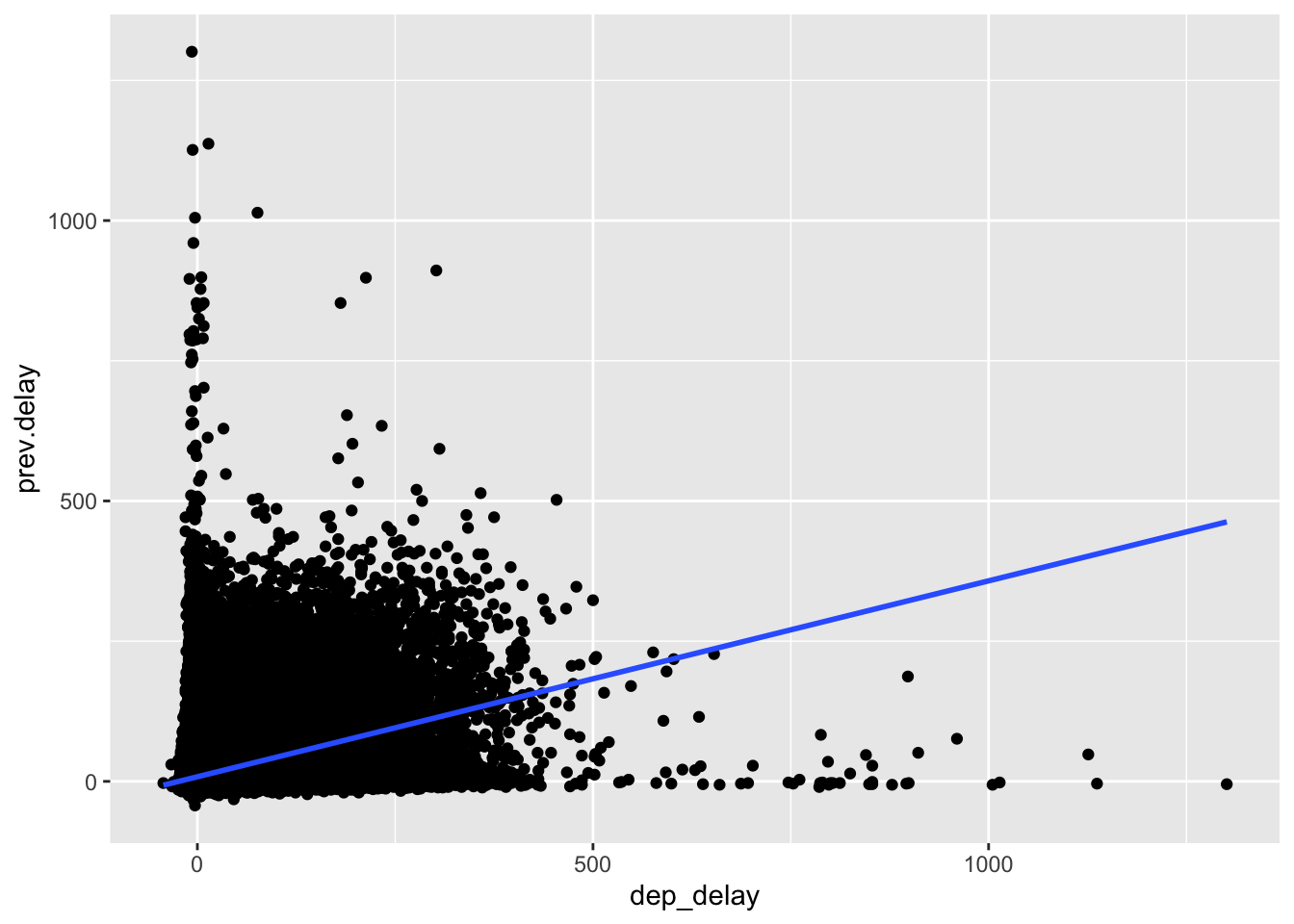
- Look at each destination. Can you find flights that are suspiciously fast? (i.e. flights that represent a potential data entry error). Compute the air time a flight relative to the shortest flight to that destination. Which flights were most delayed in the air?
flights %>%
        group_by(dest) %>%
        mutate(avg.airtime = mean(air_time, na.rm = TRUE), std.airtime = scale(air_time), n = n()) %>%
        select(year:day, dest, air_time, avg.airtime, std.airtime, n) %>%
        filter(std.airtime < -4) %>%
        arrange(std.airtime)
## # A tibble: 4 x 8
## # Groups: dest [4]
## year month day dest air_time avg.airtime std.airtime n
## <int> <int> <int> <chr> <dbl> <dbl> <dbl> <int>
## 1 2013 7 2 MSP 93 151. -4.90 7185
## 2 2013 5 25 ATL 65 113. -4.88 17215
## 3 2013 5 13 GSP 55 93.4 -4.72 849
## 4 2013 3 23 BNA 70 114. -4.05 6333- Find all destinations that are flown by at least two carriers. Use that information to rank the carriers.
- Rank by how many of the destinations a carrier flys to
pop_dest <- flights %>%
        group_by(dest) %>%
        summarise(num.carrier = length(unique(carrier))) %>%
        filter(num.carrier >= 2) %>%
        arrange(desc(num.carrier))

flights %>%
        filter(dest %in% pop_dest$dest) %>%
        group_by(carrier) %>%
        summarise(num.dests = length(unique(dest))) %>%
        arrange(desc(num.dests))
## # A tibble: 16 x 2
## carrier num.dests
## <chr> <int>
## 1 EV 51
## 2 9E 48
## 3 UA 42
## 4 DL 39
## 5 B6 35
## 6 AA 19
## 7 MQ 19
## 8 WN 10
## 9 OO 5
## 10 US 5
## 11 VX 4
## 12 YV 3
## 13 FL 2
## 14 AS 1
## 15 F9 1
## 16 HA 1